RNN: What is the difference between LSTM and GRU?
This is a series where I answer the questions my tutoring students really ask – the ones textbooks tend to skip. I teach machine learning, deep learning, statistics, and math to graduate students and working engineers.
The question. After we worked through an LSTM by hand, a student asked: “Everyone says a GRU is just a simplified LSTM. Simplified how, exactly? What did they throw out, and what does it cost?”
The fairest way to answer is to run the same prediction through both cells with the same weights and watch where the numbers diverge. So here is one day of temperature forecasting, computed twice.
The setup: predicting tomorrow’s temperature
The task, taken straight from our teaching notebook: predict tomorrow’s air temperature from today’s humidity, today’s sea-level pressure, and yesterday’s prediction. The output is a temperature index where 0.0 is freezing, 0.50 is mild, 0.77 is warm, and 1.25 is extreme heat.
Both cells share the same small weight collection, so any difference in behavior comes from the architecture, not the parameters:
Input weights (on humidity and pressure):
  candidate  W = [0.45, 0.25],  b = 0.20
  gate 1     W = [0.95, 0.80],  b = 0.65   (LSTM input gate  / GRU update gate)
  gate 2     W = [0.70, 0.45],  b = 0.15   (LSTM forget gate / GRU reset gate)
  gate 3     W = [0.60, 0.40],  b = 0.10   (LSTM output gate only)

Recurrent weights (on yesterday's output): 0.15, 0.80, 0.10, 0.25
Day 0’s input is humidity 1.0 and pressure 2.0, and yesterday’s output and memory start at zero. The actual temperature index on day 0 is 0.50.
The LSTM step: three gates, two memories
An LSTM carries two separate memories: the cell state (long-term) and the output (short-term). Three sigmoid gates decide what to keep, what to record, and what to reveal:
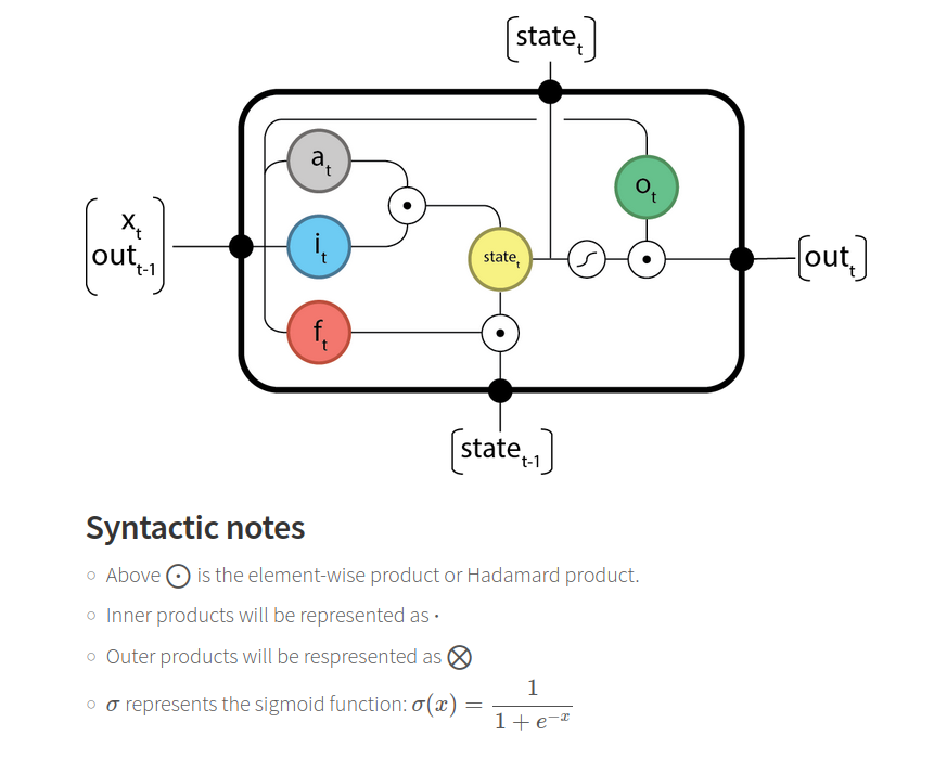
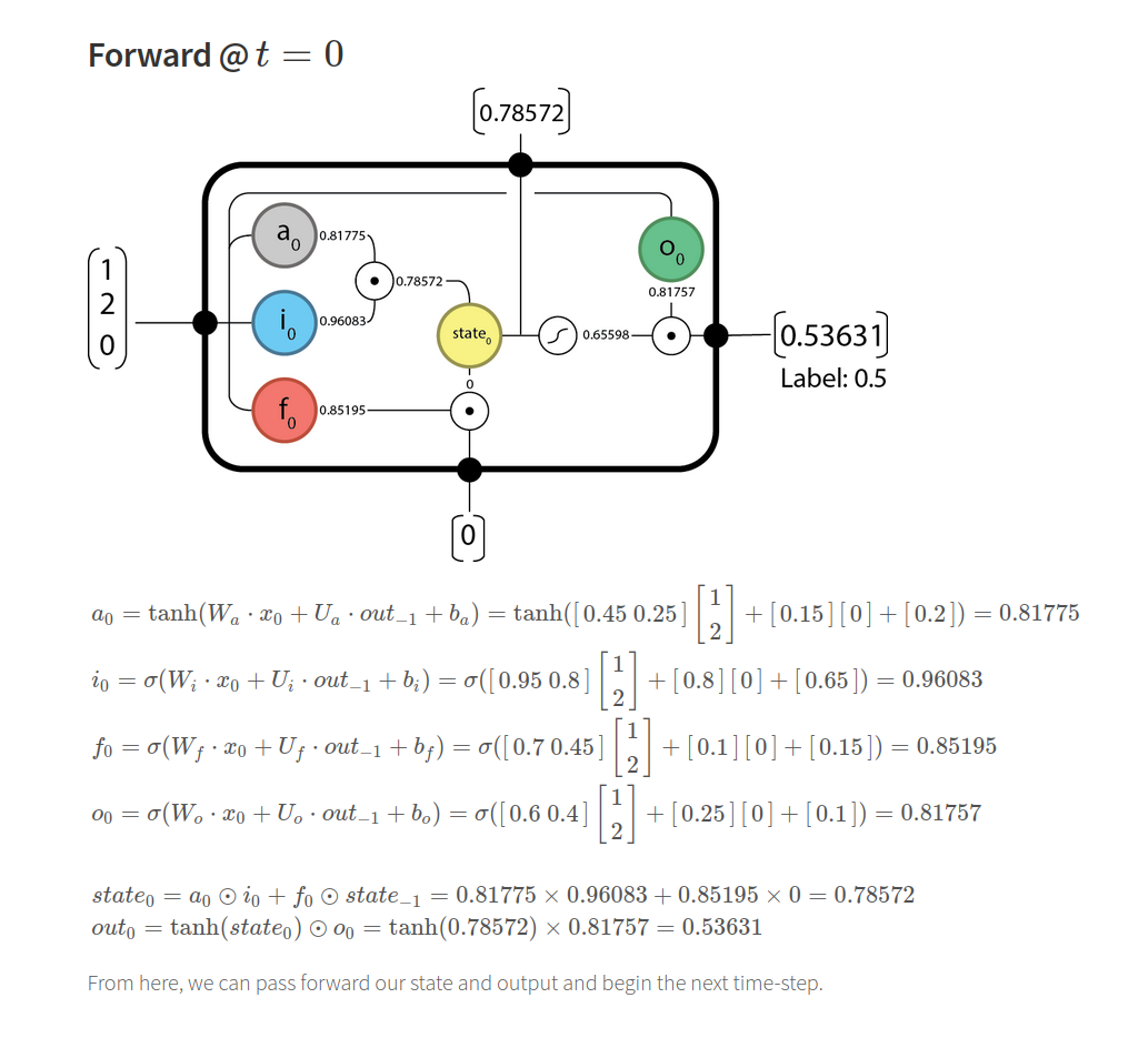
Here is the day-0 computation. I write sig() for the sigmoid function:
a_0 = tanh(0.45*1 + 0.25*2 + 0.15*0 + 0.20) = tanh(1.15) = 0.818   candidate
i_0 = sig (0.95*1 + 0.80*2 + 0.80*0 + 0.65) = sig(3.20)  = 0.961   input gate
f_0 = sig (0.70*1 + 0.45*2 + 0.10*0 + 0.15) = sig(1.75)  = 0.852   forget gate
o_0 = sig (0.60*1 + 0.40*2 + 0.25*0 + 0.10) = sig(1.50)  = 0.818   output gate

state_0 = f_0 * 0 + i_0 * a_0 = 0.852*0 + 0.961*0.818 = 0.786   long-term memory
out_0   = o_0 * tanh(state_0) = 0.818 * 0.656         = 0.536   prediction
The prediction 0.536 lands close to the actual 0.50. Notice the two-step reveal: the cell state first absorbs 96% of the candidate into long-term memory, and then the output gate decides that only 82% of that memory, squashed through tanh, becomes the visible prediction.
The GRU step: same numbers, two gates, one memory
A GRU keeps only one memory, the hidden state, which is both the long-term memory and the output. It merges the input and forget gates into a single update gate z, and adds a reset gate r that controls how much of the past the new candidate is allowed to see. There is no output gate at all:
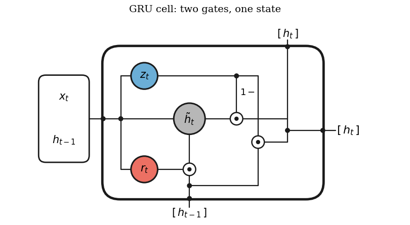
Same day, same weights:
z_0 = sig (0.95*1 + 0.80*2 + 0.80*0 + 0.65) = sig(3.20)  = 0.961   update gate
r_0 = sig (0.70*1 + 0.45*2 + 0.10*0 + 0.15) = sig(1.75)  = 0.852   reset gate
h~_0 = tanh(0.45*1 + 0.25*2 + 0.15*(r_0*0) + 0.20) = tanh(1.15) = 0.818   candidate

h_0 = (1 - z_0)*0 + z_0 * h~_0 = 0.961 * 0.818 = 0.786   prediction and memory in one
Look at that last line carefully. The GRU’s output, 0.786, is exactly the LSTM’s cell state – the number the LSTM kept hidden inside. The GRU simply publishes its whole memory as the prediction, with no tanh squash and no output gate deciding how much to reveal. That single observation is most of the answer to my student’s question.
Day 1: where the difference starts to matter
On day 1 the input is humidity 0.5, pressure 3.0, and yesterday’s output. The actual temperature index is 1.25, extreme heat. Running both cells:
LSTM:  state_1 = 0.870*0.786 + 0.981*0.851 = 1.518
       out_1   = 0.850 * tanh(1.518) = 0.772

GRU:   z_1 = 0.985,  r_1 = 0.873
       h~_1 = tanh(0.45*0.5 + 0.25*3 + 0.15*(0.873*0.786) + 0.20) = tanh(1.278) = 0.856
       h_1  = (1 - 0.985)*0.786 + 0.985*0.856 = 0.855
Both underestimate the heat, but the GRU is bolder: 0.855 against the LSTM’s 0.772. The LSTM’s output gate acts like a cautious editor between memory and prediction, while the GRU’s update gate writes 98.5% of the new candidate straight into the state it shows the world. Neither is wrong; they make different trade-offs.
So what is the actual difference?
| LSTM | GRU | |
|---|---|---|
| Gates | 3 (input, forget, output) | 2 (update, reset) |
| Memories | 2 (cell state + hidden output) | 1 (hidden state) |
| What is revealed | o * tanh(cell state) | the whole state |
| Parameter sets | 4 | 3 |
The parameter difference is real and you can measure it in two lines:
import torch.nn as nn
sum(p.numel() for p in nn.LSTM(2, 8, batch_first=True).parameters())  # 384
sum(p.numel() for p in nn.GRU(2, 8, batch_first=True).parameters())   # 288
A GRU carries 25% fewer parameters at any hidden size, which means less memory, faster training, and less data needed before it stops underfitting. The LSTM’s extra output gate buys finer control over what the memory reveals, and its protected cell state – an express lane that gradients can flow through almost untouched – is still the safer default when sequences get long and the important events are far apart. In practice the honest answer is boring: on most medium-sized problems they perform almost identically, so start with the GRU for speed and switch to the LSTM if you suspect the output gating matters.
One thing to try
Take the day-1 GRU arithmetic and force r_1 = 0. The candidate becomes tanh(0.45*0.5 + 0.25*3 + 0.20) = tanh(1.175) = 0.826, and yesterday’s 0.786 survives only through the tiny (1 - z_1) channel. Now force z_1 = 1 and watch the state get completely overwritten every day. These two knobs – how much of the past the candidate may see, and how much of the past the state may keep – are the entire GRU. Compare that with the LSTM, where f and i control the past and the present independently. That independence is what the GRU gave up for its 25% discount.
The arithmetic in this article is adapted from the teaching notebooks I use with my students, where every gate value is computed by hand before any library is allowed.
References
- Hochreiter, S., & Schmidhuber, J. (1997). “Long Short-Term Memory.” Neural Computation 9(8).
- Cho, K., et al. (2014). “Learning Phrase Representations using RNN Encoder-Decoder for Statistical Machine Translation.” arXiv:1406.1078.
- Chung, J., et al. (2014). “Empirical Evaluation of Gated Recurrent Neural Networks on Sequence Modeling.” arXiv:1412.3555.
- Olah, C. (2015). “Understanding LSTM Networks.” colah’s blog.
I tutor machine learning, deep learning, statistics, and math. If recurrent networks – or anything else – are not clicking for you, you can find me on Wyzant.