Transformer Attention: What is Attention Actually Doing?

This is a series where I answer the questions my tutoring students really ask — the ones textbooks tend to skip. I teach machine learning, statistics, and math to learners of all levels.

---

The question. A master’s student came to our session feeling stuck on attention. She had read the formula, softmax(QKᵀ/√d_k)V, three times and watched two videos about it, but she still could not answer a simple question in her own words: “What is it actually doing?”

Here is the explanation that finally made it click for her, together with the actual PyTorch code we ran in our session.

Where the confusion comes from

Most explanations start with the formula, and I think that is backwards. Attention is much easier to understand if you first see it as a three-step routine that every token performs on its own:

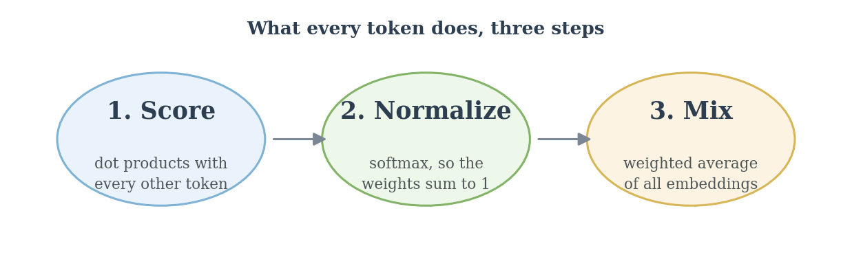
1. Score — the token compares itself against every other token by taking a dot product.
2. Normalize — the scores are turned into weights that sum to 1, using the softmax function.
3. Mix — the token takes a weighted average of everyone’s information.

The output of this routine is called a context vector. It represents the same token, but now enriched with information from the tokens that matter to it. In other words, “journey” stops being just “journey” — it becomes “journey, as understood in the context of Your journey starts with one step.”

Let’s actually run it

To make this concrete, we took six tokens with 3-dimensional embeddings. The numbers are deliberately small so that we can watch every step of the arithmetic:

import torch

inputs = torch.tensor(
[[0.43, 0.15, 0.89], # Your
 [0.55, 0.87, 0.66], # journey
 [0.57, 0.85, 0.64], # starts
 [0.22, 0.58, 0.33], # with
 [0.77, 0.25, 0.10], # one
 [0.05, 0.80, 0.55]] # step
)

It is worth pausing on what this matrix actually is, because this is the input to the whole mechanism. Each row is the embedding of one token: a short list of numbers that represents everything the model currently knows about that word. Here we use three numbers per token so the arithmetic stays readable; a real model would use 768 or 4096. So the input to attention is simply this: six tokens in, each described by a three-dimensional embedding, giving us a 6 by 3 matrix.

Step 1 — computing the scores. We let “journey” play the role of the query, and we compare it against every token with a dot product:

query = inputs[1]  # "journey"
attn_scores = torch.empty(6)
for i, x_i in enumerate(inputs):
    attn_scores[i] = torch.dot(x_i, query)
print(attn_scores)
# tensor([0.9544, 1.4950, 1.4754, 0.8434, 0.7070, 1.0865])

Step 2 — turning scores into weights. The softmax function converts the raw scores into a proper distribution that sums to 1:

attn_weights = torch.softmax(attn_scores, dim=0)
# tensor([0.1385, 0.2379, 0.2333, 0.1240, 0.1082, 0.1581])

Step 3 — building the context vector. The context vector is simply the weighted sum of all the token embeddings:

context_vec = torch.zeros(query.shape)
for i, x_i in enumerate(inputs):
    context_vec += attn_weights[i] * x_i
# tensor([0.4419, 0.6515, 0.5683])

When you repeat this for all six tokens at once, the loops collapse into just two matrix multiplications:

attn_weights = torch.softmax(inputs @ inputs.T, dim=-1)
all_context_vecs = attn_weights @ inputs
print(all_context_vecs)
# tensor([[0.4421, 0.5931, 0.5790],   # Your
#         [0.4419, 0.6515, 0.5683],   # journey
#         [0.4431, 0.6496, 0.5671],   # starts
#         [0.4304, 0.6298, 0.5510],   # with
#         [0.4671, 0.5910, 0.5266],   # one
#         [0.4177, 0.6503, 0.5645]])  # step

Now look at the output. It is another 6 by 3 matrix: six tokens out, one context vector per token, each still three-dimensional. This is the shape contract of attention, and my student found it genuinely surprising when she saw it written down. The number of tokens never changes, because attention does not add, remove, or reorder words. The width stays the same too, because each context vector is just a weighted average of the input embeddings, and a weighted average of three-dimensional vectors is still a three-dimensional vector. The only thing that changes is what each row knows: the embedding of “journey” went in describing a word in isolation, and its context vector comes out describing that same word as it appears in this particular sentence.

Here is what those weights actually look like. Every row in this heatmap is one token’s answer to the question “where should I be looking?”:

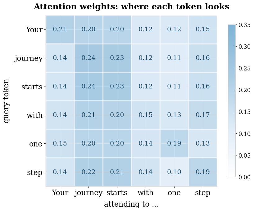
You may notice that we compared raw embeddings directly against each other here, with no learned matrices in sight. That is deliberate — it is the simplest version of the routine. My student’s very next question was about those missing matrices, and that question gets its own post.

One thing to try

Take the six-token example and change just one thing: make the embedding of “step” identical to the embedding of “journey”, rerun the code, and watch how the attention weights change. Before you run it, make a prediction first: what do you think will happen to the context vector of “Your”?

---

The code in this article is adapted from the teaching notebooks I use with my students, and it follows the progression in Sebastian Raschka’s Build a Large Language Model (From Scratch), which I highly recommend if you want to continue from here to multi-head attention and beyond.

References

1. Vaswani, A., et al. (2017). “Attention Is All You Need.” Advances in Neural Information Processing Systems 30 (NeurIPS 2017).
2. Raschka, S. (2024). Build a Large Language Model (From Scratch). Manning.
3. Tunstall, L., von Werra, L., & Wolf, T. (2022). Natural Language Processing with Transformers. O’Reilly Media.
4. How Large Language Models Work (2025).

I tutor machine learning, deep learning, statistics, and math. If attention — or anything else — is not clicking for you, you can find me on Wyzant.